7. Fields

Marey.Fields draws quantities defined over a plane: a potential, an electric field, the flow of a dynamical system. A field given as a function is sampled once onto a grid, at a resolution you state, and every mark reads the grid; ScalarGrid.create and VectorGrid.create take data that is already gridded. A sample that is not finite, as a potential is at its charge, is kept, counted and never drawn.

let dipolePotential (p: Vec2<m>) =
    let plus = Vec2.norm { X = p.X - 0.6<m>; Y = p.Y + 0.1<m> }
    let minus = Vec2.norm { X = p.X + 0.6<m>; Y = p.Y - 0.1<m> }
    (log (float minus) - log (float plus)) * 1.0<V>

let fieldXs = Grid.linear -1.8<m> 1.8<m> 108
let fieldYs = Grid.linear -1.2<m> 1.2<m> 72
let phi = Field.sampleScalar fieldXs fieldYs dipolePotential

Derivatives in the units the types work out

Field.grad, div, curl, laplacian and jacobian are differences on the grid, exact for a quadratic and second order otherwise, and their units are the types'. The gradient of a potential in volts is in V/m, and the divergence of that in V/m²:

let electricField =
    let g = Field.grad phi
    { g with U = Array.map (~-) g.U; W = Array.map (~-) g.W }

let chargeDensityOverEpsilon: ScalarGrid<m, m, V/m^2> = Field.div electricField

printfn "E is sampled at %d × %d nodes" electricField.Xs.Length electricField.Ys.Length

The marks

A scalar field draws as Field.heatmap, Field.contours (at the levels its range would be ticked at, or contoursAt stated ones) and Field.bands, each with a colorbar in the field's unit. A vector field draws as Field.quiver, an arrow per node with a key saying what one length means; Field.streamlines, evenly spaced on the page, the same lines for the same field; and Field.lic, a line-integral convolution that shows the flow at every pixel as a seeded raster. Each is computed against the panel's final scales, so the marks line up with one another, on a log axis as on a linear one. Chart.overlay puts one figure's layers over another's panel.

A dipole

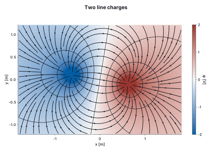
The potential of two opposite line charges on a diverging ramp, its equipotentials, and the field's lines over them. The colour range is stated, because a few nodes beside each charge would otherwise set it; the aspect is equal, because a field is read as a picture of the plane:

let dipole =
    Field.heatmapWith Theme.modern.Diverging true U.metre U.metre U.volt phi
    |> Chart.withColorDomain U.volt -2.0<V> 2.0<V>
    |> Chart.withColorLabel "φ"
    |> Chart.overlay (Field.contoursAt [| -1.5<V>; -1.0<V>; -0.5<V>; 0.0<V>; 0.5<V>; 1.0<V>; 1.5<V> |] U.metre U.metre phi)
    |> Chart.overlay (Field.streamlinesWith 18.0<px> U.metre U.metre electricField)
    |> Chart.withYLabel "y"
    |> Chart.withEqualAspect
    |> Chart.withTitle "Two line charges"

dipole

A phase space

A pendulum's state is an angle and an angular velocity, two units, so a field with one unit on both axes cannot hold it. A Flow<rad, rad/s, s> can. Its divergence is in s⁻¹, and is zero, because phase-space area is conserved. curl and laplacian need one unit on both axes, so over a phase space they do not compile: ∂ω̇/∂θ and ∂θ̇/∂ω are in different units and their difference does not exist.

Field.curl swingGrid

Phase.fixedPoints finds where the flow vanishes and classifies each point by its linearisation, with its eigenvalues in 1/'t; Phase.portrait draws the streamlines, both nullclines and the fixed points marked by kind:

let swing: Flow<rad, rad/s, s> = fun th om -> struct (om, -9.81<1/s^2> * sin (float th) * 1.0<rad>)

let swingGrid =
    Field.sampleFlow (Grid.linear -6.5<rad> 6.5<rad> 105) (Grid.linear -9.0<rad/s> 9.0<rad/s> 73) swing

let liouville: ScalarGrid<rad, rad/s, 1/s> = Field.div swingGrid

for p in Phase.fixedPoints swingGrid do
    printfn "%s" (FixedPoint.describe U.radian angularVelocity U.second p)

Phase.portrait U.radian angularVelocity swingGrid
|> Chart.withTitle "A pendulum's phase space"

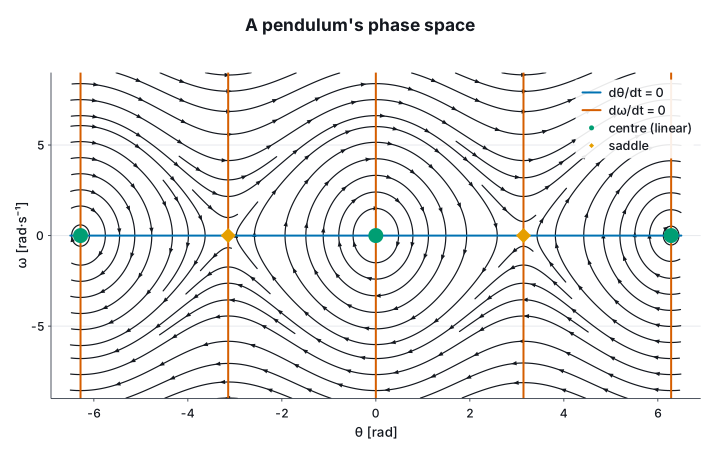
The session prints a centre at 0 and ±2π and a saddle at ±π, with eigenvalues ±3.13i s⁻¹ and ±3.13 s⁻¹: rates, so in s⁻¹ rather than Hz. A centre is a judgement, since only the nonlinear terms tell it from a weak focus, and is called one when the real part is under a thousandth of the imaginary; Phase.fixedPointsWith states another tolerance. A field that changes in time is an animation of figures, and §9 films one.