4. Axes and scales

An axis is linear unless it is told otherwise, and its domain, ticks, prefix and title come from the data and the unit. Each can be stated instead.

Scales. withXLog and withYLog put an axis on a base-10 log scale; withXScaleKind takes any of the others: ScaleKind.Log b, ScaleKind.Symlog (b, linthresh) for data that crosses zero, ScaleKind.Power p and ScaleKind.Reciprocal. A scale belongs to the axis, so a layer added afterwards is drawn on it too. withXDomain and withYDomain pin a domain. A log axis that spans three decades or fewer is ticked in plain numbers under an SI prefix; a wider one is ticked in powers of ten, 10⁻⁸, and takes no prefix.

Ticks. Ticks are chosen on a 1-2-5 ladder unless they are stated. A stated tick is in the axis's own unit, not its prefix, so it means the same on every figure, and the axis still chooses its prefix: withXTicksEvery U.metre 50e-9<m> on a nanometre axis ticks every 50 nm. withXTicksAt states the values and withXTicksNamed the labels too, which is how a band structure's axis reads X Γ X. withXMinorTicks takes MinorAuto, MinorOff, MinorCount n or MinorEvery step, and on a log axis the automatic minor ticks fill each decade.

let spectrumAxis =
    Chart.lineIn U.metre U.one [| 400e-9<m>; 700e-9<m> |] [| 0.2; 0.8 |]
    |> Chart.withXDomain 400e-9 700e-9
    |> Chart.withXTicksEvery U.metre 50e-9<m>
    |> Chart.withXMinorTicks (MinorEvery 10e-9)

let spectrumSvg = spectrumAxis |> Chart.render SvgBackend.render size
printfn "ticked every 50 nm: %b" (spectrumSvg.Contains ">450<" && spectrumSvg.Contains "[nm]")

Numbers and titles. withXPrefix writes an axis in a prefix of your choosing, Prefix.none for plain metres. withXTickFormat takes FormatFixed n, FormatPercent, FormatScientific or TickFormat.custom. An axis no prefix can carry, a dimensionless one or one with no unit stated, takes a power of ten into its title once its ticks reach 10⁶ or fall to 10⁻⁵: counts up to 4×10⁹ read y [10⁹] over ticks of 0 to 4. withXPrefix Prefix.none keeps the digits. withXReversed runs an axis from its high end, for a depth or a magnitude. withXLabel replaces the quantity in the title and keeps the unit, and withUnitStyle spells the unit in Unicode, Ascii, Latex or Siunitx. Each verb has a Y form.

A second y axis. withRightAxis takes a figure built as any other and draws its layers against an axis on the right, as matplotlib's twinx does. The two sides must agree on x, which is checked when they meet. A side with one series draws its numbers and title in that series' colour, and the legend takes both sides. withYLog sets the left side's scale and withRightYLog the right's. A second axis that reads the same quantity in other numbers is withTopAxisIn or withRightAxisIn, or a map as in §2.

A Bode plot

The response of a second-order low-pass filter with a cutoff of 1 kHz and damping ratio 0.15: its gain on a log axis, against frequency over four decades, and its phase on the right, ticked at the multiples of π/2 it passes through.

let cutoff = 1000.0<Hz>
let zeta = 0.15
let bodeFrequencies = Array.init 241 (fun i -> 10.0<Hz> * 10.0 ** (float i / 60.0))

let gain (f: float<Hz>) =
    let r = f / cutoff
    1.0 / sqrt ((1.0 - r * r) ** 2.0 + (2.0 * zeta * r) ** 2.0)

let phase (f: float<Hz>) =
    let r = f / cutoff
    -(atan2 (2.0 * zeta * r) (1.0 - r * r)) * 1.0<rad>

let halfTurn = System.Math.PI * 1.0<rad>

let phaseSide =
    Chart.lineIn U.hertz U.radian bodeFrequencies (bodeFrequencies |> Array.map phase)
    |> Chart.withName "phase"
    |> Chart.withXLog
    |> Chart.withYTicksNamed U.radian [| 0.0<rad>, "0"; -halfTurn / 2.0, "−π/2"; -halfTurn, "−π" |]

let bode =
    Chart.lineIn U.hertz U.one bodeFrequencies (bodeFrequencies |> Array.map gain)
    |> Chart.withName "gain"
    |> Chart.addVLine U.hertz cutoff
    |> Chart.withXLog
    |> Chart.withYLog
    |> Chart.withRightAxis phaseSide
    |> Chart.withXLabel "f"
    |> Chart.withYLabel "|H|"
    |> Chart.withRightYLabel "φ"
    |> Chart.withLegend LegendBottomLeft
    |> Chart.withTitle "A second-order low-pass filter, ζ = 0.15"

bode

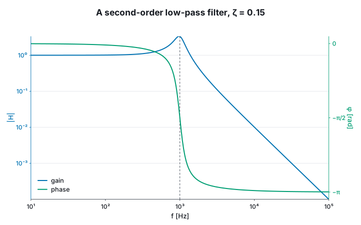
The frequency axis spans four decades, so it is ticked in powers of ten, 10¹ to 10⁵. The gain peaks at 1/(2ζ) near the cutoff and falls as f⁻² past it, two decades of gain per decade of frequency on the log-log axes. Each side's numbers are in its series' colour.